Recall from the previous lesson what a p-value is: it’s the probability of observing a value of your statistic as extreme (as far away from the null hypothesis statistic) as you in fact observed, if the null hypothesis were true.
In other words, if you’re doing a (two-sided) z test, your statistic is the mean, your null hypothesis mean is \(\mu\), and the mean you observe in your sample is \(\bar{x}\), then the p-value is the probability of getting a mean at least \(\mu - \bar{x}\) units away from the mean when randomly sampling from a normal distribution with mean \(\mu\) and standard deviation estimated by the formula for the standard deviation of a sample. (We’ll talk about that formula later, but if you want a sneak preview, check out this Khan Academy article.) If the p-value is below a predetermined level, often 0.05, then we say that there’s a statistically significant result.
Pause for a moment and ask yourself the following question: Does that mean the p-value is the probability of incorrectly rejecting the null hypothesis? Don’t go on until you have an answer, and can explain why you have that answer. This is very important.
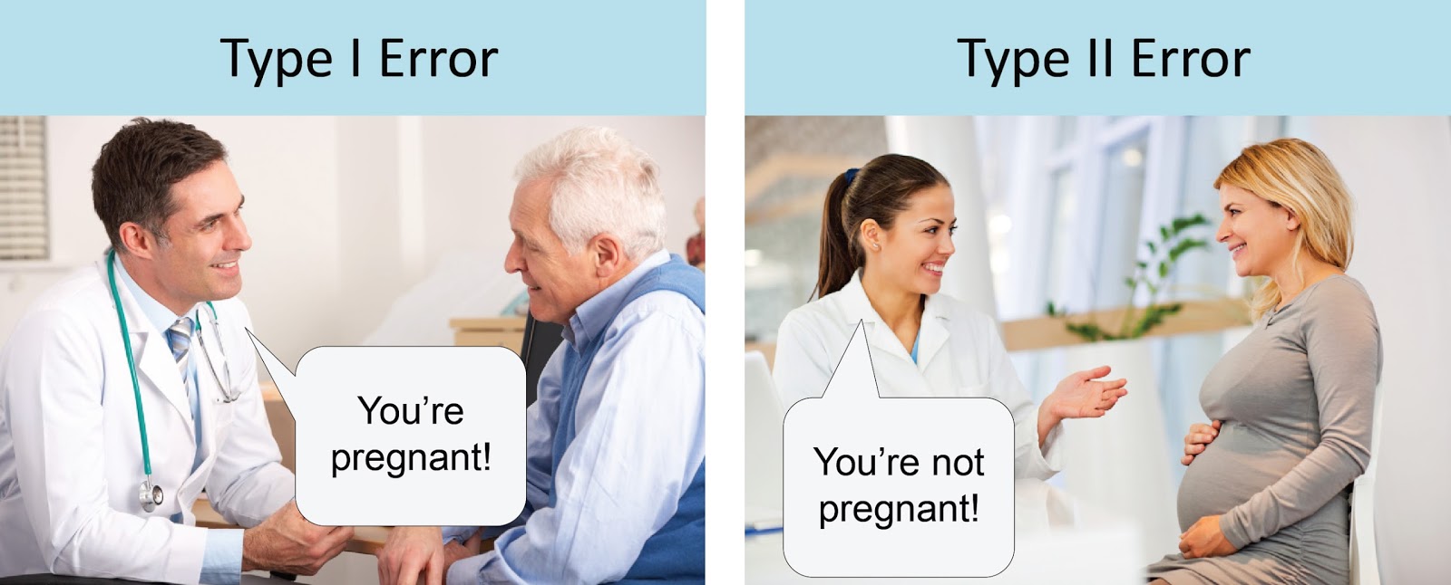
Incidentally, that’s called a "Type I error" in some circles: the error of incorrectly rejecting the null hypothesis, a.k.a. (if you’re sensible and don’t like double negatives) convincing yourself that you’re seeing a real effect when you’re not. So the question above could be rephrased: "Is the p-value the probability of making a Type I error?" A Type II error is the opposite: failing to reject the null hypothesis when you oughta, or, in other words, seeing a real effect and not realizing it. There’s a particularly good meme that captures this distinction and makes it impossible to forget:
So, what’s your answer? I’ll make some more space just to make sure you have a chance to figure it out for yourself...
.
.
.
.
.
.
.
.
.
.
.
.
The answer to my question is no. Here’s why.
If you go back to the definition I gave you of p-values, you’ll see that it’s really a conditional probability. The p value is the probability of seeing the data in your sample, conditional on the null hypothesis being true. In symbols:
But what you'd really like to know is the probability of making a Type I error--the probability of making a mistake and declaring that you’ve discovered something that isn’t. Unfortunately, that can be rephrased as the probability of the null hypothesis being true, conditional on seeing your data! In symbols:
By now, you should know that you can’t flip conditional probabilities around like that. Yet this is an incredibly common mistake--even actual statistics teachers sometimes slip up and say that the p-value is the probability of making a Type I error. It isn’t! Never say this! Never think this! Never respect anyone who does say or think it!
Here's an intuitive way of thinking about the problem. A statistically significant p-value means "if the null hypothesis were true, it would be unlikely that I'd have seen a sample that looks like that." There are some 328 million U.S. citizens, and 535 members of Congress. So, if you randomly sample 100 Americans without replacement, it's really unlikely that they're all going to be members of Congress.
How unlikely? Well, we'll want the number of possible samples of 100 members of Congress, divided by the number of possible 100-person samples: that's \({535\choose 100}\) divided by \({328,000,000\choose 100}\) which is... a lot. Let's not try and do this by hand, eh? (The parens mean, e.g., "535 choose 100"---see this explanation of the general process of reasoning here. Here's the Python function we're going to use.). This produces a probability so small that we have to use a fancy arbitrary precision math library called mpmath to get it to actually do the division.
from scipy.special import comb
import mpmath
numerator = mpmath.mpf(comb(535, 100, exact=True))
denominator = mpmath.mpf(comb(328000000, 100, exact=True))
numerator/denominator
And we get 9.0061113088164994e-584 which, in real human speak, is .9 with 584 zeroes between the decimal point and the 9... that is, significantly less likely than picking a particular atom in randomly sampling from every atom in the known universe.
So if I'm sampling Americans, it's vanishingly unlikely that that I get a sample with 100 members of Congress. \(P(Draw100Congress|Draw100Americans)\) is that tiny number up above. But it obviously does not follow that \(P(Draw100Americans|Draw100Congress)\) is small. Indeed that second probability statement is 1, or damn close to it (even though the Constitution requires members of Congress be citizens, you might imagine some incredibly unlikely event like someone getting elected to Congress after successfully deceiving the public about his/her citizenship status). In other words, I absolutely cannot infer from the unlikelihood of getting all members of Congress in my sample of Americans that it is unlikely that I had sampled Americans, given that I saw all members of Congress (Incidentally, I adapted this example from Cohen, 1994, The Earth is Round (p<.05), who in turn adapted it from Pollard & Richardson, 1987, "On the Probability of Making Type I Errors".)
Here’s why this matters. In reality, many, many studies with a "statistically significant" p-value are likely to nonetheless be Type I errors. The reason is because the actual probability of a Type I error depends on the prior likelihood that the null hypothesis was false in the first place, as well as on how likely it is that you'd see your data (in other words, on the base rate). Let’s flesh this out some more with Bayes Rule. Remember it?
As applied here, plugging in our concepts from above:
What does that mean? Well, first of all, it means that in order to even take a wild guess at how likely it is that we’re making a Type I error, we have to know how likely our null hypothesis is (in Bayesian terms, we have to have a prior probability in our heads about it). If we have strong prior reason to believe our null hypothesis--if our alternative hypothesis, or the research finding we’re trying to test out, is really crazy, then we ought to conclude that it’s more likely that we’re making a Type I error, even in the face of a statistically significant p-value. For example, if you think you’ve provided evidence for psychic abilities, as occasionally shows up in psychology journals, you should probably estimate your probability of making a Type I error as quite high, because your prior on Dr. Xavier running around somewhere controlling stuff with his miiiiiind is pretty small (or at least oughta be).
Second, you’d need to have some idea of the base rate of the data you observed in your sample (the denominator above). If it’s low, then that makes it more likely that we’re making a Type I error. Recall from our probability lesson that we can calculate that via the law of total probability as follows:
How can that value be low? Well, one important way is that \(P(DataSeen|AlternativeHypothesis)\) could be low. In other words: sure, it might be that it’s really unlikely that you’d see the data you saw if your null hypothesis were true. But what if it’s even more unlikely that you’d see the data you saw if your alternative hypothesis were true?! A low p-value means that the data you saw would come up pretty rarely in that null distribution. But what if it would come up even more rarely in every other plausible distribution? This is the lesson of our Congress example: \(P(Draw100Congress|Draw100Foreigners)\) is much smaller even than the tiny number we got for \(P(Draw100Congress|Draw100Americans)\).
What this suggests is that the construction of the hypotheses really matter. Let's return to the Congress example. Suppose my null hypothesis was "this sample was constructed from the general population of Americans," and the alternative hypothesis was "this sample was constructed from the population of people found in the U.S. Capitol on the day of the State of the Union Address." Well, now, it seems like maybe the composition of our sample tells us something useful. Because \(P(Draw100Congress|Draw100FromCapitol)\) is probably pretty big, relatively speaking.
Here’s what this all comes down to:
- Often we don’t really know these other terms that go into the Bayes Rule equation to go from p-values to probabilities of Type I errors.
- Sometimes, prior theories of how the world works (like psychic powers not being real) can give us broad guesses for those other terms, which can give us a rough idea of how confident we should be in our results. This is part of why statistics folks look down on the practice of "data-mining," a.k.a., hunting through data without a theory looking for significant results.
- The only way to be really confident that empirical results are real is by replicating them--by getting significant results again and again from different samples.
- Don’t trust that a result is real just because it has a statistically significant p-value!
- If some expert witness shows you a p-value of 0.05 and says "there's a 95% chance the null is false," you should laugh derisively at them and then fire them if they're your expert or cross examine them into oblivion if they're someone else's.
Further readings, if you’d like to learn more:
- F. Perry Wilson The P-Value is a Hoax, But Here's How to Fix it---This is an amazing concrete illustration with actual numbers of the point above about base rates. Actually, you know what? That's so good I'm going to quote it at length:
Let's say that there are 100,000 hypotheses out there -- floating in the ether. Some of the hypotheses are true, some are false (this is how science works, right?). It turns out that it's the proportion of true hypotheses that dictates how much of the medical literature is nonsense, not the p-value. Let me prove it.
Let's say that of our 100,000 hypotheses, 10%, or 10,000 are true. I may be a bit of a pessimist but I think I'm being pretty generous here. OK -- how many false positives will there be? Well, of the 90,000 false hypotheses, 5% (there's the p-value!) will end up appearing true in the study by chance alone. Five percent of 90,000 is 4,500 false positive studies. How many true positives will there be? Well, we have 10,000 true hypotheses -- but not all the studies will be positive. The number of positive studies will depend on how adequately "powered" they are, and power is usually set at around 80%, meaning that 8,000 of those true hypotheses will be discovered to be true when tested, while 2,000 will be missed.
So of our 100,000 hypotheses, we have a total of 12,500 positive studies. 4,500 of those 12,500 are false positives. That's 36%. [...]
Let that sink in. Despite the comforting nature of the 0.05 threshold for the p-value, 36% of the positive studies you read may be false.
This depends critically on the number of true hypotheses by the way. If I drop the number of true hypotheses to 5%, keeping everything else the same, then 55% of the positive studies you read are wrong. It's a disaster.
(n.b.: we'll talk about the "power" thing later on in the class.)
-
Minitab blog, "How to Correctly Interpret P Values" (Minitab is a statistical software package, and the editor of its blog is on a lovely quest to comprehensibly explain the whole p-value thing).
-
538 blog post complaining that nobody can explain p-values comprehensibly. (Mostly included because the best explanation the 538 blogger could find was from Stuart Buck... who is not only a lawyer, he was actually my law school classmate. Lawyers can understand this stuff!)
-
John Ioannidis, "Why Most Published Research Findings are False" (sort of a more complicated and less clear version of the Perry Wilson blog post above).
-
David Papineau, "Thomas Bayes and the Crisis in Science", Times Literary Supplement.